Compile the open-source electromagnetic simulation solver Palace

Palace is a parallel finite element solver developed by AWS Labs for full-wave 3D electromagnetic simulation, released under the Apache 2.0 open-source license. This solver supports full-wave frequency/time-domain simulation, eigenmode analysis, and parameter extraction for electrostatics/magnetostatics. It is compatible with platforms ranging from laptops to supercomputers and supports GPU acceleration, enabling the modeling of quantum computing hardware, RF/microwave devices, antennas, and other systems. The author previously published a brief article introducing how to compile Palace on Windows, titled Compile the electromagnetic simulation solver Palace in Windows. . Expanding upon that earlier work, this article details the compilation process more in-depth, with a particular focus on the compilation of dependent libraries. The dependent libraries discussed in this article are as follows: Hypre: A large-scale linear algebra matrix computation library, using version 2.30. MUMPS: An open-source software library for solving large-scale sparse linear systems of equations. ARPACK-NG: A library that supports complex linear matrix computations and is used for eigenvalue computation. Primarily written in Fortran, it can be compiled independently without relying on PETSc. GSLib: Used for interpolation computations in high-order spectral elements. libCEED: A linear algebra computation management framework that supports parallel computing across various CPUs, GPUs, and clusters. MFEM: A flexible, efficient, and scalable finite element discretization framework used as the core solving dependency library for Palace. System Environment and Compilers Operating System: Windows 11, 64-bit Compilers: Visual Studio 2022 Community (C++17), Intel Fortran Compiler 2022, and Intel MKL 2024. Palace Version: 0.15 Compiling Hypre Hypre is an open-source high-performance parallel linear solver library developed by Lawrence Livermore National Laboratory (LLNL) designed specifically for large-scale scientific computing and engineering simulation. Its core objective is to solve large-scale sparse linear systems of equations (in the form of Ax=b) efficiently, particularly strong at handling ultra-large-scale problems in distributed memory parallel environments. Hypre natively supports MPI parallelism, enabling it to utilize the full computing power of distributed memory architectures, such as supercomputers and clusters, and easily handle linear systems with millions or even billions of degrees of freedom. This stark advantage distinguishes Hypre from smaller solvers (e.g., Eigen). Compiling Hypre on Windows is simple. You can directly use the built-in CMake configuration file to generate Visual Studio project files, which will in turn produce the static library file. When configuring CMake, set the parameters as follows: HYPRE_WITH_MPI = ON HYPRE_USING_OPENMP = ON HYPRE_WITH_CUDA = OFF HYPRE_ENABLE_SYCL = OFF HYPRE_INSTALL_PREFIX=D:/WelSimLLC/CodeDV/3rdParty/hypre/myInstall CMAKE_INSTALL_PREFIX=D:/WelSimLLC/CodeDV/3rdParty/hypre/myInstall If the compilation proceeds smoothly, then the hypre.lib static library file will be generated. Compiling MUMPS To solve Wave Port problems, the Palace solver requires one of three direct linear algebra solvers: SuperLU, STRUMPACK, or MUMPS. MUMPS is selected as the dependent library given that the author is relatively familiar with it. MUMPS is an open-source parallel sparse direct solver library co-developed by French institutions including INRIA and CNRS. Its core objective is to solve large-scale sparse linear systems of equations (Ax=b) using the direct method. Unlike Hypre, which primarily relies on iterative methods, MUMPS computes without iteration by leveraging matrix decomposition (LU/Cholesky) via direct methods. This approach delivers higher precision and more robustness, making it particularly well-suited for solving sparse matrix problems involving asymmetric, symmetric positive definite, or indefinite matrices. MUMPS depends on BLAS/LAPACK (basic linear algebra libraries) and SCALAPACK (parallel linear algebra library). In this case, the dependency is the Intel MKL Library. The original version of MUMPS does not provide a compilation method for Windows. Instead, you can opt for the scivision/mumps version available on GitHub, which offers a CMake-based compilation approach for seamless implementation. The latest version 5.8.1 was downloaded for this example. First ensure that the environment variable contains the following configuration: MKLTOOL= C:\Program Files (x86)\Intel\oneAPI\mkl\latest Under CMake configuration, set the following parameters: MUMPS_openmp = ON MUMPS_parallel = OFF Once the Visual Studio project files are generated, compile the project to produce all static libraries of MUMPS. The generated static libraries are illustrated in the figure below. Press enter or click to view image in full size Compiling ARPACK For eigenvalue-related computations (e.g., eigenmode calculations), Palace requires a complex-number eigenvalue solver such as SLEPc or ARPACK. Since SLEPc depends on PETSc, which has a rather complex compilation on Windows, ARPACK is selected as the complex-number solver for Palace. ARPACK is an open-source library for large-scale eigenvalue and eigenvector computations, co-developed by institutions including Rice University and Sandia National Laboratories. Its core objective is to efficiently compute a subset of eigenvalues and their corresponding eigenvectors for large sparse matrices. Unlike libraries such as Hypre and MUMPS, which are designed to solve linear systems of equations (Ax=b), ARPACK focuses specifically on tackling eigenvalue problems (Ax=λx or Ax=λBx). Press enter or click to view image in full size Download ARPACK-NG from GitHub and use its built-in CMake build configuration. Set the following parameters in CMake: ICE = ON Eigen = ON Build_SHARED_LIBS = OFF Meanwhile, ensure that the environment variable contains the entry MKLTOOL= C:\Program Files (x86)\Intel\oneAPI\mkl\latest; this allows CMake to automatically locate the BLAS and LAPACK libraries within MKL. After generating the Visual Studio project files, you can directly compile the project to obtain the ARPACK static library. Compiling GSLib GSLIB is an open-source parallel sparse communication library designed to efficiently support sparse data gather/scatter communication and operators in parallel numerical simulation scenarios, such as the finite element method, spectral element method, and finite difference method. It greatly simplifies the development of parallel sparse communication and lowers the barrier to distributed memory programming. Its adaptive algorithms ensure efficient communication in large-scale parallel computing, satisfying ultra-large-scale simulation requirements. Press enter or click to view image in full size Since GSLIB does not come with CMake configuration files, it is unable to automatically generate Visual Studio project files on Windows, requiring you to create the Visual Studio project files manually. Create a new static library project named gslib-palace, and add all the source files and header files to this project. In the preprocessor definitions of the Visual Studio project, add GSLIB_USE_CBLAS and GSLIB_USE_MKL. During compilation, when the following error messages appear: unary minus operator applied to unsigned type, result still unsigned You will need to modify the code, for example, changing p[map->n].el = -(uint)1; to p[map->n].el = 0-(uint)1; This allows the compilation to succeed. Become a member When the following error message appears: potentially uninitialized local pointer variable 'h' used You will need to modify the code and initialize the pointer with a NULL value. If you receive a prompt indicating that the fgs_free function has already been defined redundantly, simply comment out the fgs_setup, fgs_free, and fgs_unique functions. Compiling libCEEM libCEED is an efficient and scalable discretization library that focuses on high-performance computational discretization based on finite element and spectral element methods. It provides a lightweight algebraic interface for linear and nonlinear operators as well as preconditioners; it supports runtime selection and optimized implementations across a variety of computing devices such as CPUs and GPUs. Compiling libCEED is the most challenging part of the entire task because libCEED does not provide CMake configuration files and contains numerous options. Coupled with the fact that Visual Studio does not support C99 syntax, extensive manual modifications to the source files are required, especially modifications related to dynamic arrays. For example, change the following dynamic array: CeedInt num_points[num_elem]; to: CeedInt *num_points = (CeedInt *)malloc(num_elem * sizeof(CeedInt)); After usage, you also need to free the array from memory at the end using the free function: free(num_points);. Certain strings containing file paths also require modification. For instance, change: *(relative_file_path) = strstr(absolute_file_path, "ceed/jit-source"); to: #ifdef _WIN32 *(relative_file_path) = strstr(absolute_file_path, "ceed\\jit-source"); #else *(relative_file_path) = strstr(absolute_file_path, "ceed/jit-source"); #endif Since Visual Studio’s support for weak functions differs from that of Linux, the weak functions in the source code need to be modified as follows: Original code: #define CEED_BACKEND(name, num_prefixes, ...) \ CEED_INTERN int name(void) __attribute__((weak)); \ int name(void) { return CeedRegister_Weak(__func__, num_prefixes, __VA_ARGS__); } #include "ceed-backend-list.h" Modified code: #ifdef _WIN32 #define CEED_BACKEND(name, num_prefixes, ...) \ CEED_INTERN int name(void) __declspec(selectany); \ int name(void) { return CeedRegister_Weak(__func__, num_prefixes, __VA_ARGS__); } #else #define CEED_BACKEND(name, num_prefixes, ...) \ CEED_INTERN int name(void) __attribute__((weak)); \ int name(void) { return CeedRegister_Weak(__func__, num_prefixes, __VA_ARGS__); } #include "ceed-backend-list.h" #endif Visual Studio does not support the __restrict__ keyword and requires it to be changed to __restrict. Other minor modifications need to be made, such as replacing popen with _popen and pclose with _pclose. Additionally, there is an environment variable setting: setenv("RUST_TOOLCHAIN", "nightly", 0), which needs to be modified as follows: char env_str[1024]; snprintf(env_str, sizeof(env_str), "%s=%s", "nightly", 0); _putenv(env_str); To reduce complexity, this compilation supports only CPU parallel computing and does not require GPU parallel support. Therefore, in the ceed-backend-list.h file, only the following functionalities need to be enabled: CEED_BACKEND(CeedRegister_Opt_Blocked, 1, "/cpu/self/opt/blocked") CEED_BACKEND(CeedRegister_Opt_Serial, 1, "/cpu/self/opt/serial") CEED_BACKEND(CeedRegister_Ref, 1, "/cpu/self/ref/serial") CEED_BACKEND(CeedRegister_Ref_Blocked, 1, "/cpu/self/ref/blocked") CEED_BACKEND(CeedRegister_Xsmm_Blocked, 1, "/cpu/self/xsmm/blocked") CEED_BACKEND(CeedRegister_Xsmm_Serial, 1, "/cpu/self/xsmm/serial") All other computing functionalities can be commented out. Upon successful compilation, the static library for libCEED will be generated. Compiling MFEM MFEM is the core solver of Palace, an open-source high-order finite element library led by the Lawrence Livermore National Laboratory (LLNL). Designed specifically for large-scale scientific computing and engineering simulation, its core objective is to provide a flexible, efficient, and scalable finite element discretization framework. MFEM also serves as a mainstream open-source finite element tool for computational fluid dynamics, electromagnetic simulation, structural mechanics, nuclear physics, and other fields. Press enter or click to view image in full size Compiling MFEM is relatively straightforward. You can generate Visual Studio project files via CMake for compilation. Set the following options to ON in CMake: MFEM_USE_MPI = ON MFEM_USE_ZLIB = ON MFEM_USE_METIS = ON MFEM_USE_LAPACK = ON MFEM_USE_LEGACY_OPENMP = ON MFEM_THREAD_SAFE = ON MFEM_USE_MUMPS = ON Generate the Visual Studio project files and compile them directly to obtain the MFEM static library. Compiling Palace At this point, all complex dependent libraries have been successfully compiled. Proceed to the final step of this project: use the built-in CMake configuration file to generate Visual Studio project files and compile Palace. Note that you should select the CMakeLists.txt file located in the palace subdirectory instead of the one in the root directory, as the latter is used for generating the SuperBuild. Set the following parameters in CMake: PALACE_WITH_ARPACK = ON PALACE_WITH_OPENMP = ON PALACE_WITH_SLEPC = OFF MPI_Fortran_WORKS = C:/Program Files (x86)/Microsoft SDKs/MPI/Include/x64 Configure the following paths: nlohmann_json_DIR = D:/WelSimLLC/CodeDV/3rdParty/nlohmann_json/json-3.12.0/myInstall/share/cmake/nlohmann_json fmt_DIR = D:\WelSimLLC\CodeDV\3rdParty\fmt\fmt-11.0.2\myInstall\lib\cmake\fmt scn_DIR = D:\WelSimLLC\CodeDV\libPack\lib\scn\cmake\scn MFEM_DIR = D:/WelSimLLC/CodeDV/libPack/lib/palace/mfem-cmake arpackng_DIR = D:\WelSimLLC\CodeDV\libPack\lib\palace\arpack-cmake\arpackng Open the generated Visual Studio project, and you will see a static library project named libpalace and an executable project named palace. If the compiler reports missing header files or the linker indicates unresolved functions during compilation, you can directly add the relevant paths and static libraries to the projects. After completing the compilation, you can run a test on palace.exe. Note that you need to place all dynamic dependent libraries (such as the MKL dynamic libraries) in the same directory as palace.exe before running it. Run a simple test case. The output shown below indicates that the compilation has been successful basically. Press enter or click to view image in full size Conclusion As open-source electromagnetic field simulation solvers are presently scarce, Palace stands out as the most feature-rich one available. As a result, Palace relies on a large number of dependent libraries, and its version is still under continuous iterations. Some of these dependencies only support Linux builds, which adds to the complexity of compiling Palace on Windows. This article documents the complete compilation process of Palace and provides a resource for the open-source community on how to build Palace for Windows. There are also other dependent libraries that are relatively easy to compile, such as Eigen, fmt, Metis, and nlohmann/json. Experienced developers can often independently build these libraries on Windows, so it is not discussed in this article. The author has included the compiled palace.exe executable file in the WELSIM installation package, so you are able to directly obtain the Windows version of palace.exe from the WELSIM installer without having to compile it yourself. This article describes the configuration of Palace for CPU multi-core parallel computing. The compilation methods for GPU-accelerated versions, such as CUDA, HIP, or SYCL, will be discussed in future articles. WelSim and the author are not affiliated with Palace, Hypre, MUMPS, ARPACK, GSLIB, libCEED, or MFEM, nor do they have any direct connections with the development teams or institutions behind these projects. The references to the names and images of these open-source software in this article are solely for the purpose of technical blog documentation and software usage guidance.

编译开源电磁仿真求解器Palace

Palace 是AWS Labs推出的一款用于全波 3D 电磁仿真的并行有限元求解器，开源许可证为Apache 2.0，求解器支持频域/时域全波、特征模、静电/静磁集总参数提取，适配笔记本到超算的多平台与 GPU 加速，可以用于量子计算硬件、射频 / 微波器件、天线等建模。 Image 笔者曾经简要介绍了如何在Windows下编译Palace的文章，参见《Windows环境下编译电磁仿真求解器Palace》一文。本文是在前文的基础上，更为详细的介绍编译过程，尤其着重介绍依赖库的编译。本文讨论的依赖库有： Hypre：大型线性代数矩阵计算包。本例使用2.33.0版本。 MUMPS：来自法国的求解大规模稀疏线性方程组的开源软件库。本例使用5.8.1版本。 ARPACK-NG：支持复数线性矩阵计算，用于特征值计算。以Fortran程序为主，无需依赖PETSc，可以独立编译。需要通过Palace提供的diff文件手动修改部分源代码。 GSLIB：用于高阶谱单元的插值计算。 libCEED：是一款线性代数计算管理终端，支持对各种CPU，GPU和集群的并行计算。本例使用0.12版本。需要手动修改源代码以通过Windows Visual Studio的编译。 MFEM：提供灵活、高效、可扩展的有限元离散化框架。本例使用4.8.1版本。是Palace的核心求解依赖库。需要通过Palace提供的diff文件手动修改部分源代码。 系统环境与依赖库 操作系统：Windows 11, 64-bit 编译器：Visual Studio 2022 Community, C++17。Inter Fortran Compiler 2022，Intel MKL 2024。 Palace版本：0.15 编译Hypre Hypre是劳伦斯利弗莫尔国家实验室 LLNL 开发的开源高性能并行线性求解器库，专为大规模科学计算和工程模拟设计。核心目标是高效求解大规模稀疏线性方程组（形如 Ax=b），尤其擅长处理超大规模、分布式内存并行环境下的问题。hypre 原生支持 MPI并行，能充分利用超级计算机、集群等分布式内存架构的算力，轻松处理数百万甚至数十亿自由度的线性系统，这是它区别于小型求解器（如 Eigen）的核心优势。 Image Windows下编译hypre并不复杂，可以直接使用自带的CMakeFile文件，生成Visual Studio的项目文件，生成静态库文件。在配置CMake时，参数如下设置： HYPRE_WITH_MPI = ON HYPRE_USING_OPENMP = ON HYPRE_WITH_CUDA = OFF HYPRE_ENABLE_SYCL = OFF HYPRE_INSTALL_PREFIX=D:/WelSimLLC/CodeDV/3rdParty/hypre/myInstall CMAKE_INSTALL_PREFIX=D:/WelSimLLC/CodeDV/3rdParty/hypre/myInstall 如果编译顺利，会生成hyper.lib静态库文件。 编译 MUMPS Palace求解器需要SuperLU, StrumPack，或者MUMPS三个直接线代求解器中的一个，才能求解Wave Port问题。由于笔者比较熟悉MUMPS，因此就选择的MUMPS求解器作为依赖库。 MUMPS是由法国 INRIA、CNRS 等机构联合开发的开源并行稀疏直接求解器库。它的核心目标是用 “直接法” 求解大规模稀疏线性方程组（Ax=b），区别于 hypre 以 “迭代法” 为主，MUMPS 用直接法通过矩阵分解（LU/Cholesky）计算出解，无需迭代，精度更高、鲁棒性更强，尤其适合求解非对称、对称正定 / 不定的稀疏矩阵问题。 MUMPS 依赖 BLAS/LAPACK（基础线性代数库）、SCALAPACK（并行线性代数库）。这里我们使用Intel的MKL库作为依赖库。 原始版本的MUMPS不提供Windows的编译方式，可以选择GitHub上的scivision/mumps版本，提供了基于CMake的编译方式，可以轻易实现编译。本例下载的是最新的5.8.1版本。 确保环境变量中含有MKLTOOL= C:\Program Files (x86)\Intel\oneAPI\mkl\latest 在CMake编译下，设置 MUMPS_openmp = ON MUMP_parallel = OFF 生成Visual Studio的项目文件后，直接编译即可生成MUMPS的所有静态库。生成的静态库如下图所示。 Image 编译ARPACK Palace在计算特征值相关的功能时，如计算Eigenmode，需要有SLEPc或者ARPACK复数求解器。由于SLEPc依赖PETSc，而PETSc在Windows下的编译较为复杂，因此就不选用SLEPc，这里选择ARPACK作为Palace的复数求解器。 ARPACK是由莱斯大学、桑迪亚国家实验室等机构，联合开发的开源大规模特征值/特征向量求解库。它的核心目标是高效计算大型稀疏矩阵的少数特征值与对应特征向量，和 hypre、MUMPS 这类求解线性方程组（Ax=b）的库不同，ARPACK 专注于处理特征值问题（Ax=λx 或 Ax=λBx）。 Image 从GitHub上下载ARPACK-ng，使用自带的CMake编译方式。确保环境变量中含有MKLTOOL= C:\Program Files (x86)\Intel\oneAPI\mkl\latest，这样CMake会自动找到MKL里的BLAS和Lapack。在CMake中设置如下 ICE = ON Eigen = ON Build_SHARED_LIBS = OFF 同时，确保环境变量中含有MKLTOOL= C:\Program Files (x86)\Intel\oneAPI\mkl\latest，这样CMake会自动找到MKL里的BLAS和Lapack。 同时，需要根据palace目录中extern/patch/arpack-ng文件夹下的diff文件，对源文件做相应修改。生成Visual Studio项目文件后，既可以直接编译得到Arpack的静态库。 编译GSLib GSLIB是一个开源的并行稀疏通信库，它专为有限元、谱元、有限差分等并行数值模拟场景，提供高效的稀疏数据聚合 – 分发（Gather/Scatter）通信与算子支持。大幅简化并行稀疏通信开发，降低分布式内存编程门槛；自适应算法保证大规模并行下的通信效率，适配超大规模仿真需求。 Image 由于GSLib并没有CMake文件，无法在Windows下自动生成Visual Studio的项目文件，需要用户自己建立Visual Studio的项目文件。新建一个静态库项目，取名为gslib-palace，并将所有的源文件和头文件添加到此项目中。 在Visual Studio的项目预处理定义中，添加GSLIB_USE_CBLAS， GSLIB_USE_MKL。 编译时，当遇到以下错误提示时： unary minus operator applied to unsigned type, result still unsigned 需要修改代码，如将 p[map->n].el = -(uint)1; 改为 p[map->n].el = 0-(uint)1; 以通过编译。 当遇到以下错误提示时： potentially uninitialized local pointer variable 'h' used 需要修改代码，给指针添加NULL初始值。 如果提示fgs_free函数已经有重复的定义。将fgs_setup, fgs_free与fgs_unique函数注释掉即可。 编译libCEEM libCEED 是一个高效可扩展的离散化库，专注于基于有限元和谱元方法的高效计算离散化。它提供轻量级代数接口，用于线性和非线性算子及预条件子，支持基于 CPU、GPU 等多种计算设备的运行时选择优化实现。 Image 编译libCEEM是整个工作的难点，由于libCEED不提供CMakeFile文件，同时含有较多的选项，同时Visual Studio不支持C99的语法，需要大量手动修改源文件，尤其是对于动态数组的修改。如将以下动态数组 CeedInt num_points[num_elem]; 修改成为 CeedInt *num_points = (CeedInt *)malloc(num_elem * sizeof(CeedInt)); 使用完成后，还需在结尾处，使用free函数，从内存中删除此数组，free(num_points)。 一些含有路径的字符串，也需要做修改。如 *(relative_file_path) = strstr(absolute_file_path, "ceed/jit-source"); 改为 #ifdef _WIN32 *(relative_file_path) = strstr(absolute_file_path, "ceed\\jit-source"); #else *(relative_file_path) = strstr(absolute_file_path, "ceed/jit-source"); #endif 由于Visual Studio对weak的函数支持方式与Linux不一样，需要对源码中的weak函数做如下修改： #define CEED_BACKEND(name, num_prefixes, ...) \ CEED_INTERN int name(void) __attribute__((weak)); \ int name(void) { return CeedRegister_Weak(__func__, num_prefixes, __VA_ARGS__); } #include "ceed-backend-list.h" 改为 #ifdef _WIN32 #define CEED_BACKEND(name, num_prefixes, ...) \ CEED_INTERN int name(void) __declspec(selectany); \ int name(void) { return CeedRegister_Weak(__func__, num_prefixes, __VA_ARGS__); } #else #define CEED_BACKEND(name, num_prefixes, ...) \ CEED_INTERN int name(void) __attribute__((weak)); \ int name(void) { return CeedRegister_Weak(__func__, num_prefixes, __VA_ARGS__); } #include "ceed-backend-list.h" #endif Visual Studio不支持__restrict__关键字，需要改成__restrict。 还有一些小范围的修改，如将popen改成_popen，将pclose改成 _pclose。有一处环境变量设定setenv("RUST_TOOLCHAIN", "nightly", 0)，需要做如下修改： char env_str[1024]; snprintf(env_str, sizeof(env_str), "%s=%s", "nightly", 0); _putenv(env_str); 为了减少不必要的复杂度，本次编译只支持CPU并行计算的内容，GPU并行无需支持，因此在ceed-backend-list.h文件中，只需要支持以下功能： CEED_BACKEND(CeedRegister_Opt_Blocked, 1, "/cpu/self/opt/blocked") CEED_BACKEND(CeedRegister_Opt_Serial, 1, "/cpu/self/opt/serial") CEED_BACKEND(CeedRegister_Ref, 1, "/cpu/self/ref/serial") CEED_BACKEND(CeedRegister_Ref_Blocked, 1, "/cpu/self/ref/blocked") CEED_BACKEND(CeedRegister_Xsmm_Blocked, 1, "/cpu/self/xsmm/blocked") CEED_BACKEND(CeedRegister_Xsmm_Serial, 1, "/cpu/self/xsmm/serial") 其余的计算功能可以注释掉。编译成功后会生成libCEEM的静态库。 编译MFEM MFEM是Palace的核心求解器，由劳伦斯利弗莫尔国家实验室（LLNL）主导开发的开源高阶有限元库，专为大规模科学计算和工程仿真设计，核心目标是提供灵活、高效、可扩展的有限元离散化框架。MFEM 也是计算流体力学、电磁仿真、结构力学、核物理模拟等领域的主流开源有限元工具。 Image 编译MFEM相对简单，可以通过CMake的方式生成Visual Studio项目文件来编译。在CMake的选项中，选择激活的选项如下： MFEM_USE_MPI = ON MFEM_USE_ZLIB = ON MFEM_USE_METIS = ON MFEM_USE_LAPACK = ON MFEM_USE_LEGACY_OPENMP = ON MFEM_THREAD_SAFE = ON MFEM_USE_MUMPS = ON 同时，需要根据palace目录中extern/patch/mfem文件夹下的diff文件，对源文件做相应修改。由于需要修改的源文件较多，需要耐心仔细，或者在Linux下先编译一遍，将自动修改好的mfem拷贝覆盖至Windows下需要编译的mfem文件夹。整个生成Visual Studio的项目文件后，直接编译，即可得到mfem的静态库。 编译Palace 至此，复杂的依赖库都已经编译完成。开始整个项目的最后一步，使用自带的CMakeFile文件，生成Visual Studio的项目文件，编译Palace。这里要注意的是，应该选择在palace子目录中的CMakeFile.txt文件，而不是根目录下的CMakeFile.txt，因为后者是用于生成Superbuild的。 CMake下设置： PALACE_WITH_ARPACK = ON PALACE_WITH_OPENMP = ON PALACE_WITH_SLEPC = OFF MPI_Fortran_WORKS = C:/Program Files (x86)/Microsoft SDKs/MPI/Include/x64 设置路径 nlohmann_json_DIR = D:/WelSimLLC/CodeDV/3rdParty/nlohmann_json/json-3.12.0/myInstall/share/cmake/nlohmann_json fmt_DIR = D:\WelSimLLC\CodeDV\3rdParty\fmt\fmt-11.0.2\myInstall\lib\cmake\fmt scn_DIR = D:\WelSimLLC\CodeDV\libPack\lib\scn\cmake\scn MFEM_DIR = D:/WelSimLLC/CodeDV/libPack/lib/palace/mfem-cmake arpackng_DIR = D:\WelSimLLC\CodeDV\libPack\lib\palace\arpack-cmake\arpackng 打开生成的Visual Studio项目，可以看到名为libpalace的静态库项目，和名为palace的可执行文件项目。如果在编译时提示找不到头文件，或者连接时缺少相关函数，可以直接在项目中添加相关路径和静态库。 Image 完成编译后，可以试运行一下palace.exe。注意使用时，需要将动态依赖库放置与palace.exe同一个文件夹下，如MKL系列的相关动态库文件。 计算一个简单算例，得到如下显示。表明编译基本成功。 Image 总结 目前可用的开源电磁场仿真求解器不多，Palace是目前功能最多的开源电磁求解器。Palace的依赖库较多，版本还在不断更新迭代，一些依赖库只支持Linux版本，增加了Windows下编译的难度。本文记录编译整个Palace的过程，同时给开源社区提供一些Windows下编译Palace的参考。 还有一些其他依赖库编译相对容易，如Eigen, fmt, Metis，nlhmann/json等。有经验的开发者可以自行在Windows下成功编译，就不在本文中赘述了。 笔者已将编译好的palace.exe可执行文件收录在WELSIM安装包中，用户也可以直接从WELSIM安装包中获得Windows版本的palace.exe，无需自己编译。 本文介绍的是CPU多核并行计算下的Palace，GPU版本的编译方法，如CUDA, HIP，或SYCL版本，会在以后的文章中讨论。 WelSim与作者不隶属于Palace, Hypre, MUMPS, Arpack, GSLib, libCEEM, 和MFEM。和Palace, Hypre, MUMPS, Arpack, GSLib, libCEEM, 和MFEM开发团队与机构没有直接关系。这里引用这些开源软件的名称和图片仅用作技术博客文章与软件使用的参考。

Generating Particles for Complex Geometries Using WELSIM

With the development of modern engineering simulation, particle-based simulation has been increasingly adopted by the industrial community. Particle-related computations and software have emerged in various fields of engineering and science. In addition to pure particle simulations, such as molecular dynamics, there are also coupled methods with continuum approaches like the finite element method, enabling more sophisticated simulations. An example is the SPH (Smoothed Particle Hydrodynamics) method, which simulates the motion of fluids and granular materials. As a result, the demands on particle simulations are also rising. Particle generation is the first and most critical step in all such simulations. Therefore, algorithms and processes for generating particles are particularly important. The author has previously discussed numerical methods for generating particles in the article titled “Automatic Generation of Simulation Particles.” Press enter or click to view image in full size Generating particles for simple geometric models, such as cubes, is not difficult. However, when the geometry becomes more complex, particle generation becomes challenging. Currently, there are not many software solutions on the market that can generate particles for arbitrary shapes. WELSIM is already capable of handling this well and can export particles as external files for use in other software. This article provides a brief introduction on how to generate particles in WELSIM. 1. Open WELSIM and Import a STEP Geometry Model In this example, a cylindrical model with a circular hole is imported. Set the geometry’s Create Particles property to True. Press enter or click to view image in full size 2. Click the Meshing Button to Automatically Generate Particles In this setup, 441 particles are generated. Press enter or click to view image in full size 3. To Increase Particle Density Modify the Maximum Size value in the mesh settings. When set to 0.01, the particle density increases. 4. Adjust Particle Display Size for Clarity When the number of particles increases, it helps to reduce their display size for better visibility. In the 3D View of the mesh object, set the Particle Size value. Here, it is set to 0.001. Now, a larger number of particles can be seen — 16,060 in total. WELSIM thus allows for easy and efficient generation of particles at any desired density. Press enter or click to view image in full size 5. Export the Particles Once particle generation is complete, export the particle file. Right-click the Mesh objectand select Export Particles from the context menu. Press enter or click to view image in full size 6. In the Export Dialog Enter the filename and choose the export format. The current version supports the VTK PolyData format. More formats will be supported in future versions. Press enter or click to view image in full size The exported file can be loaded and used by other software. For example, ParaView can be used to visualize the exported particles, as shown in the image. Press enter or click to view image in full size Conclusion This article outlines the steps for generating particles using WELSIM. Users only need to import a geometry in STEP format and, through an automatic mesh-like method, can quickly generate particles at various densities. Although a simple geometry was used here, the same process can be applied to complex models. The software also supports exporting particle data for use in other applications. The particle generation feature is already available in version 2025R3 and will continue to be improved in future releases. WELSIM has no direct affiliation with the author or the developers of ParaView. ParaView is referenced here purely as a technical example for demonstration purposes.

使用WELSIM生成复杂几何模型的粒子

随着现代工程仿真的发展，粒子仿真也越来越多的被工业届接受。粒子相关的计算和软件在各个工程和科学领域都有出现。除了单纯的粒子计算，如分子动力学计算，还有与有限元等连续介质计算方法耦合，实现更为精巧的计算。如SPH方法计算流体和沙石颗粒的运动。随之，人们对粒子计算的要求也不断提高。而生成粒子是所有计算的第一步，也是整个计算的关键一环。因此，生成粒子的算法和实现过程，就显得尤为重要了。作者曾讨论过生成粒子的数值方法，参见《自动化生成仿真粒子的方法》一文。 Image 生成简单几何模型，如立方体，的粒子并不难，但是当粒子区域轮廓变得复杂时，生成粒子就变得困难了。目前市场可以生成任意轮廓粒子的软件并不多，WELSIM已经可以很好的实现这点，并输出为外部文件，用于其他软件的计算。本文就如何在WELSIM下生成粒子，做一个简要介绍。 1. 打开WELSIM软件，并导入一个STEP几何模型。这里导入一个带有圆孔的圆柱体。并将几何体的创建粒子（Create Particles）属性设为真。 Image 2. 点击网格划分按钮，便可自动生成粒子。此设置下，生成了441个粒子。 Image 3. 如果想得到密度更高的粒子，可以修改网格设置属性中的最大单元尺寸（Maximum Size）值。当把值改为0.01时，粒子的密度会增加。 Image 4. 粒子数量增加后，为了显示更为清楚，可以调整粒子显示大小。点击网格节点的三维视图（3D View），设置粒子尺寸（Particle Size）值即可，这里设为0.001。 Image 此时，可以看到生成了更多的粒子，数量达到16,060。因此，使用WELSIM可以方便快捷地生成任意密度的粒子。 Image 5. 粒子生成工作已经完成。下一步来导出粒子文件。右键点击Mesh节点，从弹出菜单中选择导出粒子（Export Particles）。 Image 6. 在导出对话框中，输入文件名称和类型。目前已经支持了VTK PolyData格式，以后版本中，会增加更多的导出格式。 Image 导出文件可以被其他软件读取并使用。如图所示，使用ParaView读取此文件的显示结果。 Image 总结 本文介绍了如何使用WELSIM生成粒子的方法步骤。用户只需导入STEP格式的几何体，通过类似自动化网格划分的方式，快速得到各种不同密度的粒子。本文中使用的几何模型较为简单，复杂的几何体也可以同样的方式得到粒子。同时，提供了粒子数据导出功能，用户可以将生成的粒子用于其他软件的计算。粒子生成功能已经存在2025R3版中，会在后续的版本中不断增强和改进。 WelSim与作者和ParaView开发者没有直接关系。这里引用ParaView仅用作技术博客文章与软件使用的参考。

Methods for Automatic Particle Generators

Modern engineering simulation software is not only capable of analyzing continuous domains, for instance, using the finite element method (FEM) to compute structures, fluids, or electromagnetic fields, but it also has enough computational process for discontinuous particle systems. Examples include pure particle molecular dynamics, discrete element methods (DEM), smoothed particle hydrodynamics (SPH), and coupled simulations with FEM. The primary prerequisite to compute particle systems is having the ability to generate particles within a model, including data of the particle positions, shapes, and volumes. This is similar to how in finite element analysis, a mesh containing nodes and element information must first be created. When simulating particle systems, the first step is to generate the position, size, and shape of the particles. Thus, the particle generator becomes a critical component of the entire analysis system. A good particle generator should be able to quickly produce initial-state particles and generate particles according to various shapes and boundary conditions. Common automated particle generation methods are lattice structures, finite element mesh conversion, and network growth. This article discusses these well-known particle generation methods for SPH systems and their implementation mechanisms. Lattice Structures Lattice-based generation is particularly suitable for microscale materials. Typical structures include FCC (face-centered cubic) and BCC (body-centered cubic) lattices, which are often found in crystalline materials. Once the initial lattice structure is defined, the particle generator replicates this structure to fill the entire region. Press enter or click to view image in full size For this method of particle generation, the user needs to provide the boundary of the simulation domain (usually a bounding box), the particle type within each lattice, and the spacing between particles. Algorithmically, this is a straightforward approach, so it is widely applied in molecular dynamics and similar particle-based simulations. Finite Element Mesh Conversion A finite element mesh consists of nodes and elements; the element types vary depending on the model. Instances include tetrahedral and hexahedral solid meshes, as well as triangular and quadrilateral surface meshes. Since meshes can represent irregular geometries, the irregular shape stays captured once converting them into particles. In particle systems coupled with FEM, this particle generation approach allows for convenient coupling with finite element computations, as commonly seen in particle-FEM and SPH analyses. Press enter or click to view image in full size The general procedure for converting a mesh into particles involves calculating the centroid of each element and its characteristic size. These values determine the position and size of each particle. In principle, each finite element corresponds to one particle. However, because FEM meshes may be non-uniform, it may cause the resulting particle distribution to be uneven. Additional integration may be required to refine the generated particles, and boundary particles may also require special marking to enable the addition of boundary conditions in later simulations. In computational fluid dynamics (CFD), particles can also enter the simulation domain continuously through specified inflow boundaries. Currently, WELSIM supports particle generation from finite element meshes. Network-Based Generation Another common particle generation method is based on network growth, often implemented with tree and branching algorithms. Starting from an initial trunk structure, branches are allowed to grow within a fixed region according to specific rules, generating new branches (particles). By providing parameters such as a starting point, second point, segment length, gradient, and initial shape, particles can be generated iteratively. This is how new branches are created. Typically, if a new branch is too close to an existing one or belongs to the same parent particle, it is discarded. This approach incorporates randomness through stochastic processes, resulting in particle distributions with a degree of variability. Conclusion This article introduced conventionally used automated particle generation methods in simulation software. For FEM-related software, mesh-to-particle conversion is particularly practical, as the generated particles can be directly applied to FEM-coupled simulations. The general-purpose FEM software WELSIM already supports mesh-to-particle conversion, and users are able to export the generated particles to utilize in other analyses.

自动化生成仿真粒子的方法

现代工程仿真软件不仅具有分析连续介质的功能，如有限元方法计算结构、流体、或电磁场。也有增强了对非连续粒子系统的计算能力，如纯粒子的分子动力学计算，离散元，光滑粒子流体动力学（SPH），以及与有限元耦合的计算。计算粒子系统的首要条件就是能够在模型中产生粒子，包含了粒子的位置，形状，和体积大小等数据。这与有限元分析需要生成含有节点和单元信息的网格类似。 Image 在计算粒子体系时，第一步是生成粒子的位置，大小，和形状。因此，粒子生成器也就成为整个分析系统的关键部分。好的粒子生成器可以快速生成初始状态粒子，还可以根据不同的形状和边界来生成粒子。常见的自动化粒子生成方式有，晶体点阵，网络生长，和有限元网格转换。本文就讨论常见的可用于SPH系统的粒子生成方法，及其实现机理。 晶体点阵（Lattice） 使用点阵方式生成粒子是一种常见的方式，尤其适用于材料的微小尺度的计算。如材料晶体结构中常见的FCC、BCC等结构。当初始的点阵结构给定以后，粒子生成器会复制这个结构并铺满整个区域。 Image 对于此类型的粒子生成，需要用户提供整个模拟区域的边界，通常是一个矩形盒子，每个点阵中粒子类型，和粒子之间的位置。算法上，这也是一种简单直接的粒子生成方式，大量应用于分子动力学等粒子生成之中。 有限元网格转换 有限元网格是一种包含了节点与单元的数据，根据模型的不同，单元的类型也会不同。这种网格是有限元分析计算中的基础数据之一。代表性的有四面体和六面体实体单元网格，和三角形与四边形平面网格。网格可以表达不规则的形状，因此，转换成为粒子后，也可以表征不规则的形状。在与有限元结合的粒子系统中，这种粒子生成方式，能够方便与有限元计算进行耦合，如常见的粒子有限元和SPH分析。 Image 转换网格到粒子的常用方法是，获取网格每个单元的重心，和单元的直径大小。以此确定每个粒子的位置和大小。原则上每个单元会对应生成一个粒子。由于有限元网格的密度可能不均匀，以此方法生成的粒子分布也不均匀。有时需要再将生成的粒子进行均匀化处理。对于位于边界的粒子，可能还需要标记额外的内容，以方便在后续的分析中施加边界条件。如流体动力学计算(CFD)中，会在某个流入边界中不断生成粒子进入仿真区域。WELSIM已经能够根据有限元网格生成粒子的功能。 基于网络增长生成 另一种常见的粒子生成方式是通过网络增长，具体的算法上常使用树与分支的方式。初始一个树状结构的主干，允许分支在固定区域内按照一定方式生长，生成新的节点，即粒子。在输入起始点和第二个点，片段长度，梯度，初始形状等参数后。这种生成方式的核心是如何创立新的分支，通常的做法是，如果新节点与当前某个节点位置很近，或者都属于同一个父节点，则不会生成这个新节点（分支）。基于网格生成粒子的方法使用了随机数，因此生成的粒子会有一定的随机性。 Image 总结 本文介绍了仿真软件中，自动化生成粒子的常用方法。对于有限元相关的软件，网格转化为粒子的方式更为实用，可以直接将生成的粒子应用于有限元耦合计算中。通用有限元软件WELSIM已经支持了从网格到粒子的转化，用户还可以将生成的粒子导出，用于其他类型的分析。

Orthotropic Hill Plasticity Model

In the field of structural mechanics, the plastic deformation processes of many materials are anisotropic in nature. Examples include composite materials, titanium alloys, additively manufactured structures, and multiscale materials. In these cases, traditional isotropic yield criteria are no longer sufficient to accurately describe the behavior, and appropriate models are required to characterize anisotropic plastic yielding. Commonly used anisotropic yield functions include the Hill, Barlat, Banabic, and Cazacu models. Among them, the Hill model was proposed relatively early and has a wide range of applications. It performs particularly well in describing orthotropic materials and is extensively used in structural finite element analysis. hill_augmented_manufacturing The Hill model is named after Professor R. Hill, who was appointed Professor of Applied Mathematics at the University of Nottingham in 1953. His 1950 work “The Mathematical Theory of Plasticity” laid the foundation for modern plasticity theory. He is widely regarded as one of the most significant contributors to solid mechanics in the second half of the 20th century. It’s important to note that the Hill model is not the only yield criterion for orthotropic anisotropic materials. Alternatives include Barlat models with 3 or 6 parameters, or modified versions of the Hill yield criterion. This article focuses only on the classical Hill model, but similar approaches can be used to determine parameters for other yield models. The Hill model is applicable for analyzing plastic deformation in anisotropic materials and can be viewed as a generalized form of the von Mises yield criterion tailored for anisotropic behavior. It is particularly useful for orthotropic plastic materials in structural engineering applications. The Hill yield criterion is given by: hill_yield_equation For shell elements, the yield function is given by: hill_yield_equation2 Where σ represents the stress components. For 3D models, F to H are six anisotropy calibration coefficients, also known as Hill parameters, which can be determined through material experiments. For shell elements, only four parameters F to N are required. In computational mechanics, solid elements typically use yield stress ratios (or yield stresses) R11, R22, R33, R12, R13, R23 to calculate Hill parameters. To determine the yield stress ratios, the material’s yield stresses under different loading conditions must be measured: σ11, σ22, σ33 are obtained from tensile tests. σ12, σ13, σ23 are obtained from shear tests. For shell elements, Lankford parameters are used to determine the Hill parameters. A Lankford parameter rₐ is defined as the ratio of plastic strain in the plane to that in the thickness direction. For orthotropic anisotropy, rₐ can be obtained from simple tensile tests: r₀₀: tensile direction aligned with the orthotropic axis 1. r₉₀: tensile direction perpendicular to the orthotropic axis 1. Once r₀₀, r₄₅, r₉₀ are measured, the Hill parameters can be calculated. Higher Lankford values indicate better formability. Most finite element analysis software requires the user to input either R values or Lankford parameters for the Hill model. Once these are specified, the Hill yield criterion equation can be fully determined. Support for the orthotropic Hill model in WelSim The complexity of the Hill model lies in parameter input and solving the orthotropic nonlinear behavior. The general-purpose simulation software WESLIM supports transient analysis involving the Hill model. The free material editing software MatEditor supports Hill material model input. Currently, MatEditor supports three types of orthotropic Hill plastic material models and can generate OpenRadioss material input scripts: Law32, Law73/74, and Law93. mateditor_hill_orthotropic Conclusion The Hill model effectively describes orthotropic yield behavior, especially in tension-compression directions and in scenarios with minimal shear deformation. It can also be used to model the mechanical behavior of metallic lattice structures in additive manufacturing. Hill parameters can be determined via R or Lankford parameters. When these parameters are unavailable from experiments, they can be approximated using curve fitting methods. WelSim already provides support for the Hill model and can be integrated with OpenRadioss for transient simulations involving orthotorpic plastic deformation. WelSim and authors have no direct affiliation with developers of OpenRadioss. References to OpenRadioss here are solely for technical blogging and software usage discussion.

正交各项异性Hill 塑性模型

在结构力学领域，很多材料的塑性变形过程是各项异性的，如复合材料，钛合金，增材制造结构，多尺度材料等。这时传统的各项同性屈服准则就无法准确描述此过程，需要有合适的模型来描述各项异性塑性屈服，常用的各项异性屈服函数有：Hill 系列、Barlat 系列、Banabic和 Cazacu等。其中，Hill模型是提出较早，且应用范围广。尤其是在描述正交各向异性材料，Hill模型有着很好的表现，被广泛应用于结构有限元计算中。 Image Hill塑性模型是以R. Hill教授命名的，他在1953年被任命为诺丁汉大学应用数学教授。于1950年发表的《塑性数学理论》奠定了塑性理论的基础。被广泛认为是20世纪下半叶固体力学基础最重要的贡献者之一。 Hill模型并不是描述正交各项异性屈服的唯一准则，例如3参数或者6参数的Barlat本构模型，或者修改版的Hill屈服准则。本文仅对经典的Hill模型进行讨论，其他屈服模型也可以采用类似的方法进行确定。 Hill适用于各项异性的塑性变形分析。可以看作是用于各项异性屈服行为的von Mises屈服准则的通用形式。在实际的结构工程中，常用于正交各项异性的塑性材料。 Hill 的屈服准则如下： Image 对于壳单元，屈服函数如下 Image sigma是应力分量，对于三维模型，F-H为六个各向异性校准系数，又称作Hill参数，可以通过材料实验得到。对于壳单元，只需要F-N 4个参数。 在计算上，固体单元使用 屈服应力率 （或屈服应力）R11, R22, R33, R12, R13, R23来计算Hill参数。为了得到屈服应力率，材料在两种载荷工况下的屈服应力需要被测量。其中，屈服应力sigma11, sigma22, sigma33从拉伸测试中获得。屈服剪应力 sigma12, sigma13, sigma23从剪切测试中获得。 对于壳单元，会使用Lankford参数组来决定Hill参数。Lankford参数r_a是 平面上与厚度方向上塑性应变的比值。对于正交各项异性，r_a可以从简单的拉伸测试中获得。比如r00 从拉伸测试中，载荷方向与正交第一方向一致。r90的载荷方向与正交第一方向垂直。一旦Landford参数r00, r45, r90获得，便可以计算得到Hill参数。Landford数值越大，表示材料有更好的延展性。 在大多数有限元分析软件中，Hill模型要求用户输入R或者Landford参数。通过确定R或者Landford参数，即可确定Hill屈服准则方程。 WelSim对正交各项异性Hill模型的支持 Hill模型的复杂性在于模型参数的输入，和正交各项异性的非线性的求解。通用仿真软件WELSIM支持含有Hill的瞬态动力学计算，免费的材料编辑软件MatEditor支持Hill材料模型的输入。目前MatEditor已经支持了三种正交各项异性Hill塑性材料模型，并支持生成OpenRadioss的材料卡片Law32， Law73/74和Law93。 Image 总结 Hill模型可以描述材料的正交各项异性屈服行为。尤其是在拉压方向，以及剪切变形较小的场合，Hill模型也可以描述金属增材点阵结构的力学行为。 Hill参数可以通过R或者Landford参数确定，当这些参数无法从实验中获得时，也可以通过曲线拟合的方法近似得到。 WelSim已经对Hill模型有了一定支持，能够联合OpenRadioss进行含有各向异性塑性变形的瞬态动力学计算。 WelSim与作者和OpenRadioss开发者没有直接关系。这里引用OpenRadioss仅用作技术博客文章与软件使用的参考。

Running OpenGL-based applications in a sandbox/virtual machine

Windows Sandbox is a built-in virtual machine in the Windows operating system that allows users to test and run uncertain applications. The sandbox is seperate from the host OS, so applications can run safely in isolation. It is temporary; once closed, all software, files, and states within the sandbox are deleted. Each time the sandbox is launched, a brand-new instance is created. Unlike other virtual machines like VirtualBox, launching Windows Sandbox doesn’t require installing or purchasing a separate OS, which is a significant advantage. However, the sandbox is only available on Windows Professional or Enterprise editions. When running OpenGL-based software in the sandbox, display issues may arise. This is because Windows Sandbox does not natively support OpenGL. If an application depends on OpenGL but does not include the necessary OpenGL libraries, issues can occur such as a missing main interface. For example, MatEditor, a free engineering simulation material editor from the WelSim suite, may not display its main window the first time it is opened in the sandbox. This is because the required OpenGL libraries in the sandboxed OS are absent. The fix is straightforward — simply add the OpenGL libraries to MatEditor. Download the Mesa OpenGL library from GitHub. The project name is mesa-dist-win. 2. Choose the appropriate version for your operating system and build type. In this case, the release-msvc version is selected. 3. Extract the files, open the extracted directory, and type cmd in the address bar to open a command prompt. Then, run the perappdeploy.bat file. 4. The command line will launch and display relevant information. Press any key to continue. 5. Follow the prompts by inputting the executable file folder: C:\Program Files\WELSIM\MatEditor, the executable file name: runMatEditor.exe, and selecting the processor architecture: x64. 6. The OpenGL library is now added to MatEditor. You can re-run the application, and the main window should now display correctly. Conclusion This article uses MatEditor as an example to demonstrate how to resolve OpenGL library dependency issues in Windows Sandbox. The same method applies to other environments lacking OpenGL support, such as Windows systems running in VirtualBox. Besides MatEditor, other WelSim products such as the general simulation software WELSIM and the free curve fitting tool CurveFitter are also based on OpenGL and will require similar configuration when used in the sandbox. WelSim and its developers are not directly affiliated with OpenGL, Windows, Linux, VirtualBox, or Sandbox. References to these technologies are solely for technical blog purposes and software usage guidance.

沙盒/虚拟机中运行基于OpenGL的应用软件

Windows沙盒（Sandbox）是Windows操作系统中自带的虚拟机。对于不确定的应用程序，可以先在沙盒里测试运行。沙盒与当前的操作系统隔离，可以安全地在隔离状态下运行应用程序。沙盒是临时的，关闭后，系统将删除所有软件和文件以及状态。 每次打开应用程序时，都会获得沙盒的全新实例。打开沙盒系统无需安装或购买一份新的操作系统，这是相对于VirtualBox等虚拟机来说一个优势，但是只有在Windows专业版或企业版才有沙盒功能。 在沙盒环境下运行含有OpenGL的软件时，可能会遇到一些显示问题。由于沙盒环境下没有对OpenGL的原生支持，因此，当应用软件基于OpenGL但不包含OpenGL依赖库的时候，会出现显示的问题，如没有主界面等现象。WelSim系列的MatEditor是一款免费的工程仿真材料编辑软件，当在沙河中首次打开时，可能会无法显示主窗口，是由于沙盒的操作系统中没有OpenGL的相关库文件。 Image 解决方法很容易，只需要为当前的MatEditor程序添加OpenGL的库即可。 1. 从GitHub上下载Mesa的OpenGL库，项目名称为mesa-dist-win。 Image 2. 选择对应的操作系统和编译方式版本。这里选择的是release-msvc版本。 Image 3. 解压后，在解压目录中输入cmd，进入命令行模式。并运行perappdeploy.bat文件。 Image 4. 会进入命令行模式，并显示相关信息。按下任意键后。 Image 5. 根据提示，分别输入可执行文件的文件夹C:\Program Files\WELSIM\MatEditor。可执行文件的名称runMatEditor.exe。选择处理器构架为x64。 Image 6. 为MatEditor添加OpenGL库文件的工作已经完成。可以再次运行MatEditor应用。主窗口与界面完美显示。 Image 总结 本文通过以MatEditor软件为例，介绍了在Windows沙盒中解决和OpenGL依赖库有关的问题。此方法同样适用没有OpenGL支持的操作系统环境，如Virtual Box中的Windows系统。除了MatEditor，WelSim系列下的通用仿真软件WELSIM，和免费的曲线拟合软件CurveFitter也都基于OpenGL，因此在沙盒环境下，也需要做类似配置。 WelSim与作者和OpenGL, Windows, Linux, VirtualBox, SandBox等开发机构没有直接关系。这里引用OpenGL, Windows, Linux, VirtualBox, SandBox仅用作技术博客文章与软件使用的参考。

Finite Element Analysis of Plastic Roll Forming

Roll forming, also known as cold roll forming, is an industry-wide process used to manufacture and form metal. Through successive deformation, it shapes the metal workpiece into specific profiles using a series of forming rollers arranged in sequence. This forming method offers high production efficiency, reduced waste, and enhanced product strength. Roll forming is widely applied in industrial sectors such as automotive manufacturing. Simulation of roll forming is a common type of finite element analysis (FEA). With this analysis, one can predict the degree of deformation of the workpiece, the stresses and strains it undergoes, as well as determine the roller dimensions and operating speeds required for success. Since this type of analysis involves nearly all aspects of structural calculations, such as multi-load steps, nonlinear plasticity, various types of contact algorithms, rigid body dynamics, and both solid and shell elements, it is considered one of the most copmlex and difficult-to-converge models in structural analysis. An analysis of roll forming not only places high pressure on the solver, but also on the skill of its pre- and post-processors. The general-purpose engineering simulation software WelSim, when combined with the powerful open-source FEA solver OpenRadioss, can effectively simulate various plastic forming and forging processes. This article demonstrates how to perform a roll forming simulation from a practical perspective. Analysis Steps 1. Open WelSim and set units. In this case, we use the kg-mm-s system. 2. Create a new aluminum alloy material named myPlastic, with the following properties: Density: 2.7e-6 kg/mm³ Young’s Modulus: 70 GPa Poisson’s Ratio: 0.33 Johnson-Cook Plasticity Properties: Initial Yield Stress: 300 MPa Hardening Constant: 360 MPa Hardening Exponent: 0.08 After editing the material parameters, close the material window to proceed with the analysis. 3. Create a new FEM project and set the analysis type to Explicit Transient Structural Analysis in the Properties window. 4. Import the geometry model as shown below: In this assembly, the bottom two rotating rollers transport the workpiece, while the top roller presses down on the workpiece. The workpiece is a square tube with chamfered corners. The cross-section of the tube is shown below: For the three cylindrical rollers, set them as Shell structures. The Material is Structural Steel; Thickness is 1 mm. Set the Integration Points property to 3, and set the Rigid Body property to true. For the deformable square tube workpiece, define it as a Solid structure, and assign the aluminum alloy created in Step 2 to the Material. 5. In the Mesh Settings window, set the Maximum Element Size to 10 mm. WelSim automatically meshes based on geometry type. The square tube is meshed with solid elements. The thin-walled rollers are meshed with shell elements. 6. In the Contact property windows, this model defines three contact pairs: two frictionless, and one frictional. 6.1 The first contact pair is frictional; it is between the bottom front roller and square tube. The friction coefficient is 0.9 to provide driving force as the roller rotates. 6.2 The second contact pair is frictionless and is between the rear bottom roller and tube. 6.3 The third contact pair is frictionless and is between the top pressing roller and tube. 7. Now, define this analysis to be multi-step. In the properties of Study Settings object, set up 3 load steps. The end times for each step are: 0.04s, 0.045s, and 0.1s. Set the solver to OpenRadioss, or leave it as the default (Program Controlled). When performing explicit structural dynamics, WelSim defaults to OpenRadioss as the solver. 8. Next, define four boundary conditions for this analysis. 8.1. The Displacement boundary is set for the top roller. The roller moves downward 20 mm at a constant speed during first load step, then holds position. 8.2. A Constraint condition is set for top roller to prevent some rotation during simulation, only Z direction translation and X axis rotation are allowed. 8.3. Now, define the constraints for the bottom rollers to only allow rotation around the X-axis by setting X to False. 8.4. The last boundary condition is the angular velocity of the front bottom roller, which is set to a speed of 200 rad/s, and it starts in the second load step. 9. Now it’s time to solve the Model. You can simply click the Solve button to begin the computation. If it’s your first time using WelSim with OpenRadioss locally, you’ll need to download the OpenRadioss solver and configure its path in WelSim’s Preferences. 10. After computation, you can view results by clicking the Answer object. The Table and Chart display energy and kinetic quantities over time. These quantities include: Contact energy, External work, Internal energy, Kinetic energy, Mass, Momentum, etc. 11. You also can add result objects like stress, strain, displacement to evaluate the specific results of the domain. To see the deformation, you need to enable the Show Deformation property in the 3D View tab. The figure below displays the von-Mises stress contour; the Table and Chart display how stress evolves over time. WelSim also supports the generation of animation, just click the record button in the Chart window to create an animation of the 3D view. The example animation is shown here: https://www.youtube.com/watch?v=-38eodbujns Conclusion This article demonstrates how to build and analyze a plastic roll forming simulation using a real-world example. OpenRadioss proves to be a powerful tool for transient structural analysis. Paired with WelSim's convenient pre- and post-processing capabilities, OpenRadioss becomes easier to use and integrate. WelSim acts as both the pre- and post-processors in this case, efficiently generating complex input scripts and directly reading the result files for display. WelSim seamlessly integrates with the OpenRadioss solver. The geometry and test files used in this article are open-sourced and available in WelSim's official test case repository: 🔗 https://github.com/WelSimLLC/WelSimAutoTests WelSim has no direct affiliation with the developers of OpenRadioss. References to OpenRadioss are for technical blog and software usage purposes only.

塑性辊压成型的有限元仿真

塑性辊压成型又称冷弯成型，是工业中常用的金属制造与成型方式。是通过顺序配置的多道次成形轧辊，把金属工件不断进行变形，以制成特定形状。这种成型方式生产效率高，节约材料，增加产品强度，广泛应用于如汽车生产等工业部门。 Image 辊压成型的仿真也是常见的有限元分析类型。通过这种分析，可以预测工件的变形程度，承受的应力应变情况，以及所需要辊子的尺寸和运转速度。由于此类分析几乎涉及了结构计算的所有因素，如多载荷步，塑性非线性变形，各种类型的接触算法，刚体动力学，和各种实体与板壳单元。可以说是结构分析中最复杂，最难以收敛的模型之一。这不仅对求解器提出很高的要求，也对前后处理器也需要比较完善的功能。 通用工程仿真软件 WelSim，在结合强大的开源瞬态求解器OpenRadioss后，可以很好的模拟各种塑性成型等锻造过程。本文就从实际操作角度，演示如何进行滚动压铸成型的仿真分析。 分析步骤 1. 打开WelSim主界面，并设置单位。这里，我们设置kg-mm-s。 Image 2. 建立一个新的铝合金材料，并命名为myPlastic，设置的属性分别如下。 密度：2.7e-6 kg/mm3。杨氏模量：70 GPa。泊松比：0.33。 Johnson-Hook塑性属性，初始屈服应力：300 MPa。硬化常数: 360 MPa。硬化指数: 0.08。 Image 编辑完成材料参数后，关闭材料窗口。进行后续分析操作。 3.新建一个FEM项目工程，并在属性窗口中，设置为显式瞬态结构分析。 Image 4. 导入几何模型，如下图所示。 Image 底部有两个可转动辊轴，用于传送工件。上转辊用于下压工件。工件为方管结构，四角有倒角。方管的横截面如下图所示。 Image 对于3个圆柱形辊子，在属性窗口中设置为壳体结构，材料为结构钢，厚度保持1mm不变，积分点保持3个不变，同时将刚体选项设置为真。如下图所示， Image 对于受挤压成型的方管工件，定义为实体结构，并赋予在第2步创建的铝合金塑性材料。 Image 5. 网格划分。将最大单元尺寸设置为10mm。WelSim会自动根据几何类型进行划分单元。方管会使用实体单元网格划分。薄壁滚轴是使用壳单元划分。 Image 6. 添加接触。本算例中，需要添加3对接触对，其中两个无摩擦接触对，一个有摩擦接触对。第一个接触对是底部第一滚轴与方管的接触，设置为有摩擦，同时摩擦系数为0.9。之所以设置成有摩擦，是为了在滚轴转动时，摩擦力能将方管向一个方向传递。 Image 第二个接触对是底部第二滚轴与方管的接触，定义为无摩擦接触。如下图所示， Image 第三个接触对是顶部的压辊与方管的接触，同样定义为无摩擦接触。 Image 7. 在Study Settings节点中设置多载荷步分析。由于分析工况的需要，我们将载荷步设置为3步，每一个载荷步的结束时间分别是0.04s, 0.045s, 0.1s。将求解器设置OpenRadioss或者保持默认的自动选择求解器。WelSim在进行显式结构动力学计算时，会默认使用OpenRadioss求解器。 Image 8. 设置边界条件。这里要设置四个边界条件，用于完成整个分析中所需的约束与载荷。 8.1 对顶部的辊子设置位移边界条件。上辊在第一个时间步内匀速下压20mm, 并在之后的过程中保持在这个位置。 Image 8.2 对上辊设置约束边界条件。目的是防止上辊在接下来的计算中产生转动。因此，只允许Z方向和X轴方向运动。 Image 8.3 对底部两个辊子都施加约束边界条件。只允许以X轴方向的转动。 Image 8.4 对底部前端的辊子施加以X为轴的旋转角速度，用于传动方管。角速度的大小为200 rad/s，从第二个载荷步开始旋转辊子。 Image 9. 设置完成后，即可以点击求解按钮，进行计算。如果是在本地第一次使用WelSim和OpenRadioss的联合求解，还需要下载OpenRadioss求解器至本地，同时在WelSim的首选项中进行简单配置，输入OpenRadioss的目录地址。即可联立求解。 Image 10. 计算完成后，点击答案节点，会在表格与曲线窗口，显示整个时间历程下，各种能量和动能的分布。这些量包括，接触能量，外部做功，内能，动能，质量，和动量等。如下图所示。 Image 11. 还可以添加如应力、应变、位移等结果节点，评价后即可得到三维云图显示。当需要打开变型显示时，可以在三维显示属性窗口中，将显示变形属性设置为真。即可看到方管变形和位移后的状态。同时，表格和曲线窗口显示整个应变随时间变化的状况。 Image WelSim还支持快速生成动画，用户可以点击曲线窗口上的录像按钮，即可生成3D视图窗口中的动画文件。本算例的应力结果动画如下所示。 总结 本文通过一个实例，演示了如何建立塑性辊压模型，并得到计算结果。OpenRadioss被证明是一款功能强大的瞬态结构动力分析软件，通过WelSim便捷的前后处理能力，使得OpenRadioss的更加易于使用。WelSim在本例中，作为前后处理工具，快速生成包含复杂内容的求解文件，同时可以直接读取结果文件并显示，体现了和OpenRadioss求解器无缝整合的功能。 本文所用的几何文件和测试文件已经开源，并共享在 WelSim的官方测试库中，https://github.com/WelSimLLC/WelSimAutoTests。 WelSim与作者和OpenRadioss开发机构没有直接关系。这里引用OpenRadioss仅用作技术博客文章与软件使用的参考。

WELSIM 2025R2 releases to enhance structural dynamics

 The general-purpose engineering simulation software WELSIM has released its latest version 2025R2 (internal version number 3.1). Compared with the previous one, version 2025R2 contains many new features and enhancements, which can better support various types of engineering analysis, especially structural dynamics.

Enhance support for OpenRadioss

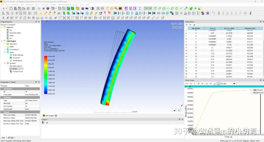
The new version improves the pre- and post-processing support for the OpenRadioss solver. Through support of thermal stress commands, WelSim now has the ability to solving thermal stress problems. The reading and display of contact force results have also been added. More functions such as remote displacement boundary conditions have been implemented, too.

In the material editing module, new material properties applicable to OpenRadioss have been added, such as damage plasticity (LAW23), brittle plasticity (LAW27), honeycomb structure (LAW28), Swift plasticity, Ramberg-Osgood plasticity, etc. The existing thermal expansion and specific heat material properties can output the solver command in OpenRadioss format. The independent material editing software MatEditor has also added the same function.

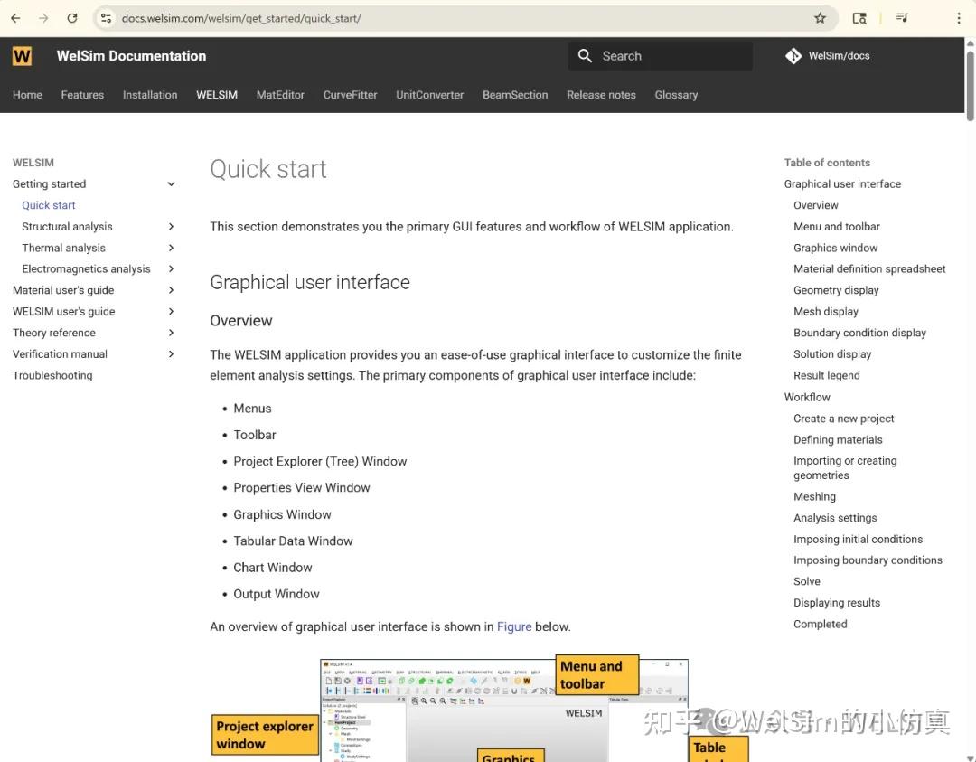
Open source WelSim’s documentation

All help documents of WelSim are open source now. This is another open source intelligent asset of WelSim, after the official website and automated testing cases. Not only can users can submit document updates about WelSim, but they can also use this framework to build online help documents for their own products. The documents are currently open source on GitHub at https://github.com/WelSimLLC/welsim-docs.github.io.

Other enhancements and upgrades

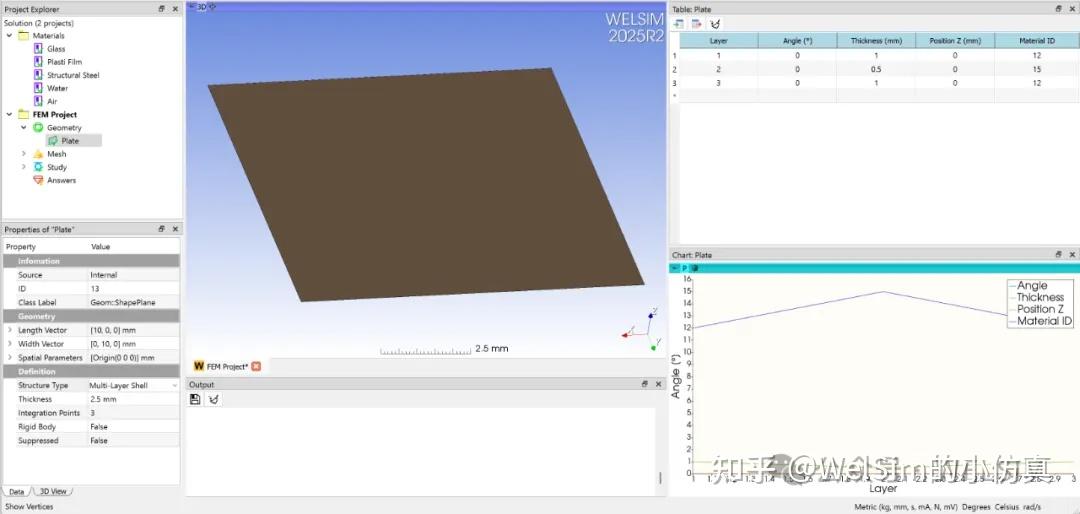
The new version has even more features and improvements. For one, WelSim now supports pre-processing of multi-layer shell structures. There have also been advancements to improve user experience: the application window title displays the full path name of the current project file, and users can now drag and drop STEP geometry files. Additionally, the CFD solver SU2 has been upgraded to the latest version 8.2. And other enhancements and upgrades.

WELSIM and the author are not affiliated with OpenRadioss, SU2. The use of OpenRadioss, SU2 is for reference in this technical blog post and software usage only.

WELSIM发布2025R2版本，增强结构动力学计算

通用工程仿真分析软件WELSIM发布了最新的2025R2版本（内部版本号3.1）。相对于上一个版本，2025R2版本含有许多新的功能与增强，能够更好地支持各种类型的工程仿真CAE分析，尤其是瞬态结构动力学分析功能。

增强对OpenRadioss的支持

新版本增强了对OpenRadioss求解器的前后处理支持。通过支持对热应力命令的支持，使得WelSim具备了求解热应力问题的功能。增加了对接触力结果的读取与显示。支持了远端位移边界条件等新功能。

在材料定义与编辑模块，增加了可应用于OpenRadioss的新的材料属性，如损伤塑性（LAW23），脆性塑性(LAW27)，蜂窝结构(LAW28)，Swift塑性，Ramberg-Osgood塑性等。已有的热膨胀与特热材料属性可以输出OpenRadioss格式的求解器命令。独立材料编辑软件MatEditor，也同步增加了相同功能。

开源WelSim帮助文档

开源了WelSim的全部帮助文档。这是继开源官方网站和自动化测试后，又一次开源WelSim相关的知识资产。用户不仅可以提交关于WelSim的文档更新，也能够以此框架，建立自己产品的在线帮助文档。目前文档开源在GitHub上，地址为https://github.com/WelSimLLC/welsim-docs.github.io

其他增强与升级

此外，新版本还有其他功能与提升。如支持了多铺层板壳结构的前处理。软件窗口标题显示当前项目文件的全路径名称。支持拖拽导入STEP几何文件。升级SU2求解器到最新的8.2版本。等其他增强与提升。

WelSim与作者不隶属于OpenRadioss和SU2, 和以上开发团队与机构没有关系。这里引用OpenRadioss, SU2 仅用作技术博客文章与软件使用的参考。

Finite element analysis of plastic deformation using WELSIM

 Plastic deformation refers to the process in which a structure experiences external stress beyond its yield limit, transitioning from elastic deformation to plastic deformation. This process is also referred to as elastoplastic deformation. Plastic deformation is commonly seen in industrial applications, such as the formation of various sheet metal and die casting of automobile bodies. In a professional engineering context, engineers aim to avoid plastic deformation in structures to prevent material failure. As a result, plastic analysis is very common in structural finite element analysis.

The general-purpose engineering simulation software WELSIM already supports plastic analysis. This article gives an overview of the plastic analysis features in the current version from a practical software usage perspective.

From a computational standpoint, plastic deformation is a nonlinear process in a material’s constitutive relationship. Therefore, the software must have the capabilities to solve nonlinear problems. WELSIM uses FrontISTR as its implicit solver and OpenRadioss as its explicit solver. Users can also use other solvers such as CalculiX and Elmer, which will be covered in future articles. This article focuses on the FrontISTR and OpenRadioss solvers.

Most of the complexity in plastic deformation lies in the material behavior. Therefore, considerable effort is required for the material data input and editing. With the diversity of plastic models, the front-end interface also needs to be robust. WELSIM provides a user-friendly material editor and a fully consistent, free standalone material software called MatEditor. Currently, 25 plastic-related and 12 creep-related material properties are supported. Each property has its own parameters and editing method.

Using multilinear hardening as an example, the figure below demonstrates how to define an elastoplastic material. Basic parameters are entered:

• Density: 7.8e-7 kg/mm³
• Young’s modulus: 206.9 GPa
• Poisson’s ratio: 0.29

Plastic stress-strain relationship data:

• Strain: {0, 0.05, 0.1, 0.2, 0.3, 0.4, 0.5}
• Stress: {450, 608, 679, 732, 752, 766, 780} MPa

Static elastoplastic analysis

For static nonlinear finite element analysis, the computation is essentially implicit. Nonlinear material deformation is solved using the Newton iterative method. In the project settings, you can retain the default “Static Structural Analysis” type.

Because plastic deformation is a nonlinear process, multiple sub-steps can be set in the analysis. In this example, 25 sub-steps are used.

The other analysis settings are almost identical to those in elastic analysis.

After setting boundary conditions and running the simulation, you will obtain common results like stress and displacement. For simple models, the stress results can also reflect the plasticity.

WELSIM uses FrontISTR as the default solver for static structural analysis. Supported default plastic models include:

• Bilinear
• Multilinear
• Swift
• Ramberg-Osgood
• Kinematic Hardening

Transient elastoplastic analysis

For WELSIM’s transient structural analysis, it is recommended to use explicit method with OpenRadioss as the solver. OpenRadioss is an excellent open source solver for structural dynamics, known for reliable results, and it supports a wide variety of plastic models.

In the project settings, set the analysis type to “Transient” and enable “Explicit” analysis.

In transient analysis, it’s often necessary to set the physical time for each load step and time step. As shown in the figure:

• Total time: 0.07s
• Time step: 0.0001s

After defining boundary conditions and running the computation, results can be obtained.

Supported plastic models for explicit transient analysis are given below:

1. LAW2 (PLAS_JOHNS) — Density + Isotropic Elasticity + Johnson-Cook
2. PLAS_ZERIL — Density + Isotropic Elasticity + Zerilli-Armstrong
3. LAW22 (DAMA) — Density + Isotropic Elasticity + Johnson-Cook + General Damage
4. LAW27 (PLAS_BRIT) — Density + Isotropic Elasticity + Johnson-Cook + Orthotropic Brittle Failure
5. LAW28 (HONEYCOMB) — Density + Honeycomb
6. LAW32 (HILL) — Hill
7. LAW36 (PLAS_TAB) — Density + Isotropic Elasticity + Rate-Dependent Multilinear Hardening
8. LAW44 (COWPER) — Cowper-Symonds
9. LAW93 (ORTH_HILL) — Orthotropic Hill
10. LAW48 (ZHAO) — Zhao
11. LAW49 (STEINB) — Steinberg-Guinan
12. LAW52 (GURSON) — Gurson
13. LAW57 (BARLET3) — Barlet3
14. LAW78 — Yoshida-Uemori
15. LAW79 (JOHN_HOLM) — Johnson-Holmquist
16. LAW84 — Swift-Voce
17. LAW103 (HENSEL-SPITTEL) — Hensel-Spittel
18. LAW110 (VEGTER) — Vegter

Note: WELSIM does not include OpenRadioss in its installation package. Users need to download OpenRadioss separately and configure its directory in WELSIM’s preferences before using it for the first time.

Conclusion

This article introduces how to use WELSIM to perform finite element analysis (FEA) on structures with plastic materials. With its excellent material editing module and powerful solvers like OpenRadioss and FrontISTR, users can carry out plastic structural analysis and obtain results quickly.

WelSim and author are not directly related to the OpenRadioss, FrontISTR, Elmer, or CalculiX development team. The reference to OpenRadioss FrontISTR, Elmer, or CalculiX is only used here for technical blog and software usage references.